Analytic description of "Think Bayes"

Introduction

Think Bayes

The book "Think Bayes" solves various problems with Bayesian inference without using mathematical (analytic) calculations. Instead of mathematics, it uses python codes to achieve the result. It gives a good insight on what's happening behind the mathematics. However, for those who have a mathematical background, analytic expressions may give yet another insight and help to understand. So in this article, I'll show analytic calculations on some example problems in the book.

Chapter3 - The locomotive problem

The prior distribution is:

where is the number of locomotives the railroad owns, and is the upper bound of the possible numbers.

If you observed a locomotive with the number , the likelihood is:

Then the posterior distribution becomes:

The normalization constant is:

Hence,

Especially, when ,

This matches with the result of Figure 3-1.

As another case, if you observed three locomotives with the number , the likelihood is:

Then the posterior distribution becomes:

The normalization constant is:

　

Hence,

Now, the mean of the posterior is:

　

Especially, when and ,

This matches with the result in the book.

From this calculation, you can see that the posterior depends only on the largest number you observed.

Chapter6 - The Price is Right problem

We will calculate from Player1's view point with the following notation.

: Actual price
: Guessed price
: Bid price
: Actucal price of the opponent (Player2)
: Bid price of the opponent (Player2)

We have the following data from past results.

: Distribution of actual price for Player1
: Distribution of actual price for Player2
: Set of price differences for Player1
: Set of price differences for Player2

Now we make some assumptions.

First, Player1's guess contains some error around the actual price. We assume the gaussian distribution with mean and the same variance as the past price differences. That is:

where is a sample variance of and is a gaussian distribution.

Then using as a prior distribution of the actual price, and using guessed price as an observed data, the posterior distribution becomes:

Where is a normalization constant. Based on this posterior distribution of the actual price, Player1 needs to take some strategy to decide the bid price because there are the following trade-offs. (It's not wise to simply bid the maximum likelihood price.)

1. If , the probability of overbid becomes large.

2. If , the probability of losing to Player2 (Player2 makes more accurate bid) becomes large.

So, assuming that Player1's bid is , we calculate the probability of winning as:

where is a probability that Player2 overbids which is a constant inferred from . is a probability that Player2 makes less accurate bids, that is, . This is also inferred from for a fixed value of .

Hence the expected gain with a bid for some fixed actual price can be calculated as:

Finally, using the posterior distribution of the actual price, the expected gain (without knowing the true price) is:

　

As an example, we'll have a rough estimation for and . (According to the result in the book (Figure 6-4), the expected gain for this range will be constant around 7500.)

From the numeric result of the posterior (Figure 6-3 in the book), this has a peak around . Hence,

From the inferred probability of Player2's error (Figure 6-2 in the book), we can see the fact that and (because Player2 doesn't make an error larger than 20000, and our assumption is ). As a result:

This matches with the expected result. Yeah!

Chapter12 - Interpreting SAT scores

Before going into analysis, let's recap some basics of the beta distribution. The beta distribution gives the probabilistic distribution of variable within the range with two parameters . Suppose that we repeat some independent experiment which gives one of two results A or B for each trial (like a coin flip). The possibility of having A from a single trial is unknown, but if the number of A is and the number of B is , the distribution of can be estimated as .

For example, if , the distribution of is which has a smooth mountain like shape with a peak at .

The mathematical definition is given as:

If we use the beta distribution for a prior of variable , and likelihood is given by the binomial form , the posterior becomes the beta distribution again. This can be easily understood from the following calculation.

This indicates that the posterior is given by

Now, let's go ahead with the problem. We'll evaluate the possibility of giving a correct answer to one question. From the past results (Figure 12-1 in the book), the mean of is around 0.5. So we assume that prior of is given by .

If a student has the ability , what is the probability density that he/she gives correct answers to questions from questions in total? It is given by the binomial distribution, that is, .

Hence, form the discussion about the beta distribution, the posterior of is given by .

Based on this result, we can compare the ability of two students with the following data.

　Total number of questions:

　The number of correct answers for Student1:

　The number of correct answers for Student2:

The joint probability density of Student1's ability and Student2's ability is given by:

.

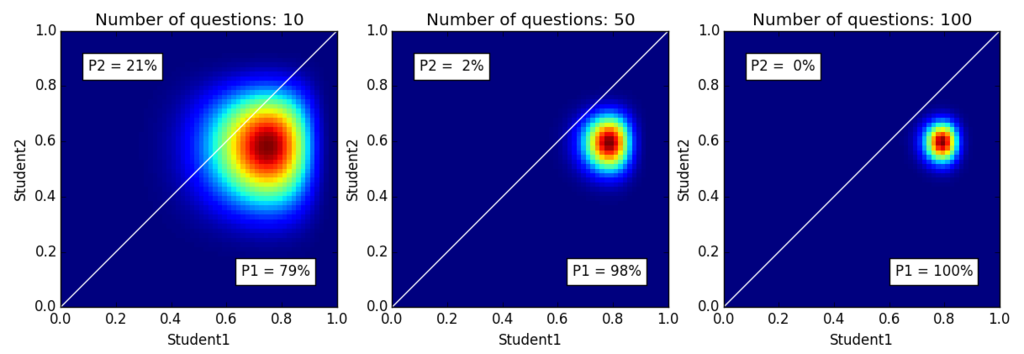
We can draw a heatmap (like Figure 12-5 in the book) using python for some specific cases. We take the following three cases:

The ratio of correct answers (score of the exam) is the same for all cases. But you can see a difference from the actual heatmap below:

P1 and P2 is a ratio of the total probability in each triangle. P1 is the probability that Student1 gets better score than Student2 in the next exam. It shows that we have more confidence in their abilities if students give answers to more questions.

Here's the python code to draw the heatmap.

import matplotlib.pyplot as plt
from pandas import DataFrame
import numpy as np
from scipy.stats import beta

# Resolution
R = 60

# (Max, Student1, Student2)
Dataset = [(10,8,6), (50,40,30), (100,80,60)]

def post(m, k, p):
    return beta(a=2+k,b=2+m-k).pdf(p)

def drawmap(d, subplot):
    M,N1,N2 = d
    X = np.linspace(0,1,R)
    Y = np.linspace(0,1,R)
    field = DataFrame(np.zeros(shape=(len(X),len(Y))))
    p1 = 0.0
    p2 = 0.0
    for x, xval in enumerate(X):
        for y, yval in enumerate(Y):
            p = post(M, N1, xval)*post(M, N2, yval)
            field.ix[y,x] = p
            if x == y:
                p1 += p * 0.5
                p2 += p * 0.5
            elif x > y:
                p1 += p
            else:
                p2 += p
    z = p1 + p2
    p1 = p1 * 100 / z
    p2 = p2 * 100 / z

    subplot.set_title("Number of questions: %d" % M)
    subplot.set_xlabel("Student1")
    subplot.set_ylabel("Student2")
    subplot.imshow(field.values, 
        extent=(0,1,0,1), origin='lower', interpolation='nearest')
    subplot.plot([0,1], color='white')
    subplot.text(0.1, 0.9, 'P2 = %2.0f%%' % p2,
        horizontalalignment='left', verticalalignment='top',
        bbox={'facecolor':'white', 'alpha':1, 'pad':10})
    subplot.text(0.9, 0.1, 'P1 = %2.0f%%' % p1,
        horizontalalignment='right', verticalalignment='bottom',
        bbox={'facecolor':'white', 'alpha':1, 'pad':10})

# Main
if __name__ == '__main__':
    fig = plt.figure()
    for i, d in enumerate(Dataset):
        subplot = fig.add_subplot(1,3,i+1)
        drawmap(d, subplot)
    fig.show()

Chapter 14 - The Geiger counter problem

First we calculate the posterior of an emission count under a fixed emission rate . In other words, all probabilities are conditioned with .

The prior of is given by the Poisson distribution:

--- (1)

The likelihood of counting particles is given by the Binomial distribution:

--- (2)

Hence, the posterior of becomes:

--- (3)

Then we calculate the posterior of .

The prior of is a uniform distribution between .

The likelihood of counting particles is given by marginalizing with :

　(from (1)(2))

Hence, the posterior of becomes:

(for )

　 --- (4)

where we cut off the summation by for the sake of numeric calculation performed later.

Finally, the posterior of which is marginalized with is:

--- (5)

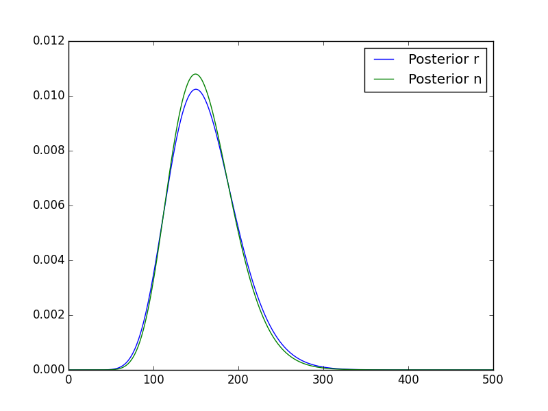
The result (3), (4) and (5) can be evaluated with a numeric calculation using python as below.

Here's the python code to draw it.

import matplotlib.pyplot as plt
import numpy as np
from scipy.stats import binom, poisson

f = 0.1
k = 15

def postn_conditioned_r(ns, r): # (3)
    result = np.zeros(500)
    ns = np.arange(1, 501)
    result = poisson(r).pmf(ns) * binom(p=f,n=ns).pmf(k)
    result /= result.sum()
    return result
    
def calc_postr(rs):             # (4)
    result = np.zeros(500)
    for n in range(1, 501):
        result += poisson(rs).pmf(n) * binom(p=f,n=n).pmf(k)
    result /= result.sum()
    return result

def calc_postn(ns, post_r):     # (5)
    result = np.zeros(500)
    for r in range(1, 501): 
        result += postn_conditioned_r(ns, r) * post_r[r-1]
    result /= result.sum()
    return result

# Main
if __name__ == '__main__':
    fig = plt.figure()
    subplot = fig.add_subplot(1,1,1)

    rs = np.arange(1, 501)
    post_r = calc_postr(rs)
    subplot.plot(rs, post_r, label="Posterior r")

    ns = np.arange(1, 501)
    post_n = calc_postn(ns, post_r)
    subplot.plot(ns, post_n, label="Posterior n")

    subplot.legend(loc=0)
    fig.show()

Chapter15 - Lions and tigers and bears

First, we calculate the prevalence conditioned with .

: Prevalence of each animal.

where

The prior of is given by the Dirichlet distribution with parameter :

Likelihood of finding animals, say, lions, tigers and bears, is:

where

The tricky summation comes from the fact that we don't know which of animals correspond to what we found (lions, tigers and bears). Hence we count all possible combinations.

Then the posterior becomes:

--- (1)

where is a normalization constant depending on . Explicitly:

　 --- (2)

For the last part, I used the fact that the integrand is symmetric with permutations of .

Now we calculate the distribution of hyperparameter .

The prior is a uniform distribution between .

The likelihood marginalized with is:

　

For the last part, I used the fact that the integrand is symmetric with permutations of .

Now, the posterior of becomes:

　 --- (3)

Since analytic evaluation of this integral is difficult, we use the numeric sampling with python code later. We assume that we have calculated (3) at the moment.

Finally, we evaluate the posterior of prevalence for each animal by marginalizing with . Since we don't know which of corresponds to each animal, I'll sum up all possibilities. In the case of lion:

where . The integration with is to get marginalized with the prevalences of other animals.

And is a probability where corresponds to . Using (1), it becomes:

Putting them together, we have:

　

　

where we used the symmetry of the integrand again. Finally, by substituting (2):

　

　

　 --- (4)

We've done it! Here's the python code to calculate (3) and (4).

import matplotlib.pyplot as plt
import numpy as np
from scipy.stats import beta
from scipy.special import binom as binom_coef

d = np.array([3,2,1])
N = d.sum()

Iter_num = 4000

def calc_post_n(ns):
    total = np.array([0.0]*len(ns))
    for n in ns:
        if n < len(d):
            continue
        for i in range(Iter_num):
            ps = np.random.gamma(shape=1, scale=1, size=n)
            ps /= ps.sum()
            total[n] += binom_coef(n,len(d)) * (ps[:len(d)] ** d).prod()
    total /= total.sum()
    return total

def calc_post_p(ps, i, post_n):
    total = 0.0
    for n in range(len(d), 31):
        xs = np.ones(n, dtype=np.int)
        for j in range(len(d)):
            xs[j] += d[j]
        total += post_n[n] * beta(a=xs[i],b=(xs.sum()-xs[i])).pdf(ps)
    return total

# Main
if __name__ == '__main__':
    fig = plt.figure()
    subplot1 = fig.add_subplot(1,2,1)
    subplot2 = fig.add_subplot(1,2,2)

    ns = np.arange(0, 31)
    post_n = calc_post_n(ns)
    subplot1.plot(ns[len(d):], post_n[len(d):], label="Posterior n")
    subplot1.set_xlim(0,30)
    subplot1.legend(loc=0)

    ps = np.arange(0, 1, 0.01)
    post_ps = {}
    for i in range(len(d)):
        post_ps[i] = calc_post_p(ps, i, post_n)
        subplot2.plot(ps, post_ps[i],
            label="Posterior p%d (%d)" % (i, d[i]))
    subplot2.legend(loc=0)

    fig.show()

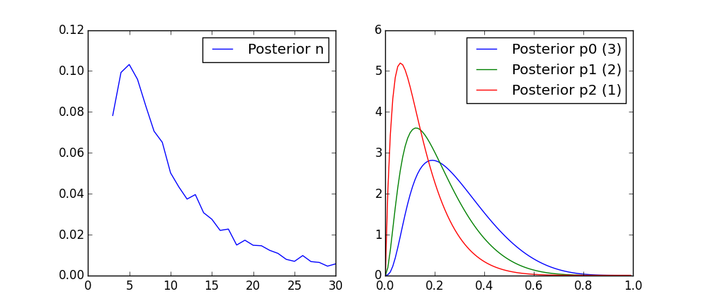
The result for is as below:

The posterior of is the same as figure 15-2 in the book.

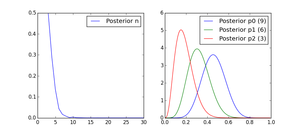
What happens if we found more animals with the same ratio? The following is the result for .

We have more confidence on the number of species now.